Power Law Distributions and Model-fitting Approaches

A power law distribution has a heavy tail. The following simulation results depict the form of a power law distribution. In this example, the value of is 3.6, the minimum value is 8.9, and the sample size is 75. The histogram shows the values that resulted from the simulation run, while the red line shows the theoretical distribution. Note that a few simulation values are much, much larger than the rest. To preview some results to be presented later, the distribution of debitage size in lithic reduction experiments looks similar. Such similarity is suggestive but not definitive.

As discussed previously, linear regression analysis has sometimes been used to evaluate the fit of the power law distribution to data and to estimate the value of the exponent, . This technique produces biased estimates, which the next simulation results illustrate. In the simulation, a random number generator produced a sample of numbers drawn from a power law distribution at a particular value of . I then analyzed this artificial data set using the linear regression approach described by Brown (2001) and using maximum likelihood estimation through a direct search of the parameter space. For a simple power law distribution, the maximimum likelihood estimate could also be found analytically. I used a direct search approach, however, in anticipation of using this approach for more complex mixture models. I repeated the random number generation and analysis 35 separate times for several different combinations of and sample sizes. The following histograms show the estimates for using the linear regression analysis and maximum likelihood estimation to find that value. In this particular case, was set to 3.6 in the random number generator, the minimum value was set to 8.9, and the sample size was 500.

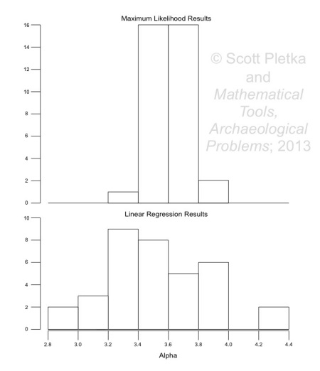
The histograms clearly suggest that the maximum likelihood estimates center closely around the true value of alpha, while the regression analyses skew to a lower value. The simulations that I performed at other parameter values and sample sizes displayed similar results. Other, more extensive simulation work also supports these impressions (Clauset et al. [2009] provides these results as part of a detailed, comprehensive technical discussion). Consequently, I used maximum likelihood estimation to fit probability distributions to data in the subsequent analyses.

References cited

Brown, Clifford T.
2001 The Fractal Dimensions of Lithic Reduction. Journal of Archaeological Science 28: 619-631.

Clauset, Aaron; Cosma Rohilla Shalizi; and Mark E. J. Newman
2009. Power-law distributions in empirical data. SIAM Review 51(4): 661-703.

© Scott Pletka and Mathematical Tools, Archaeological Problems, 2013

Tags: maximum likelihood, mixture models, power law distribution